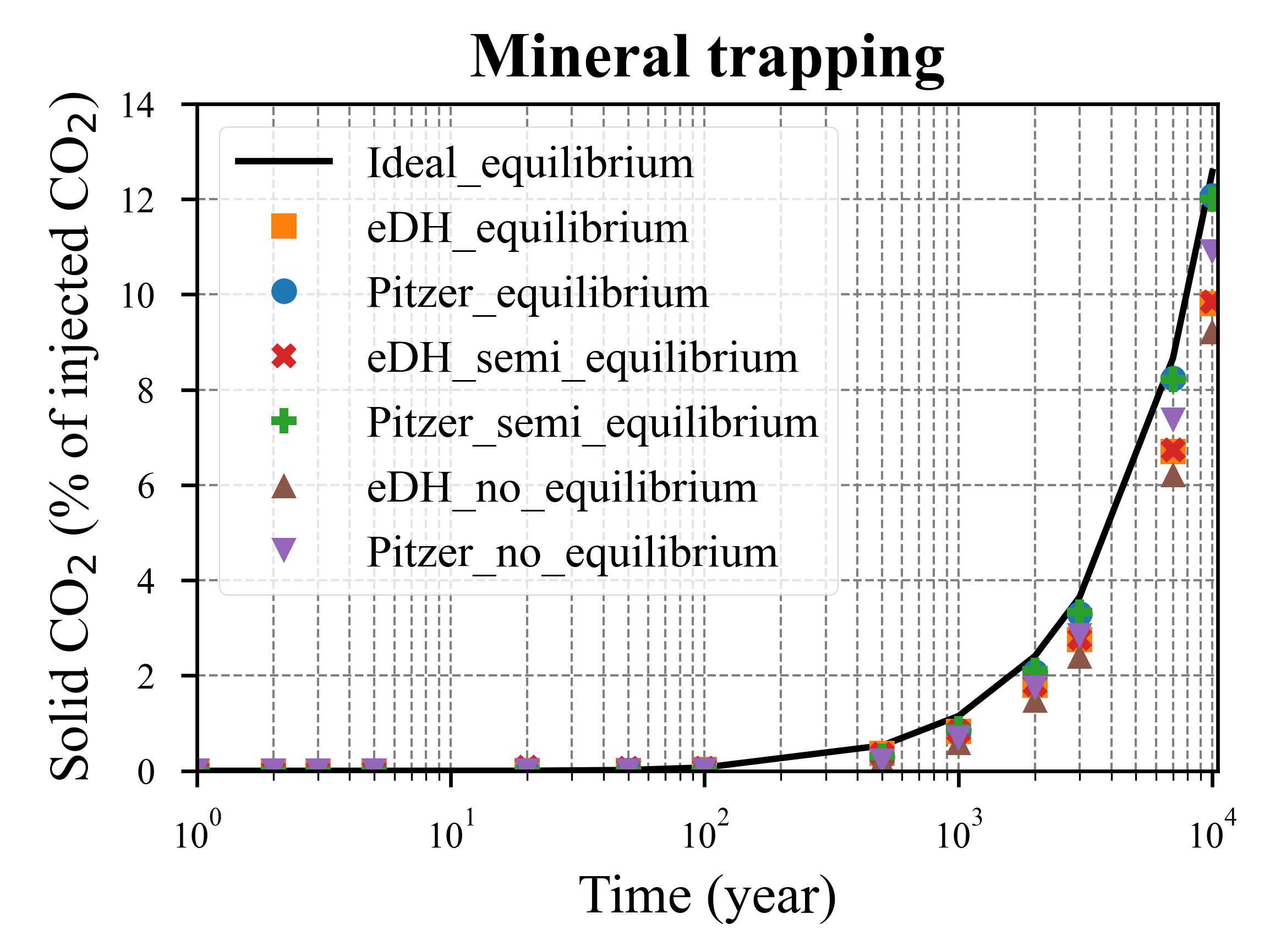
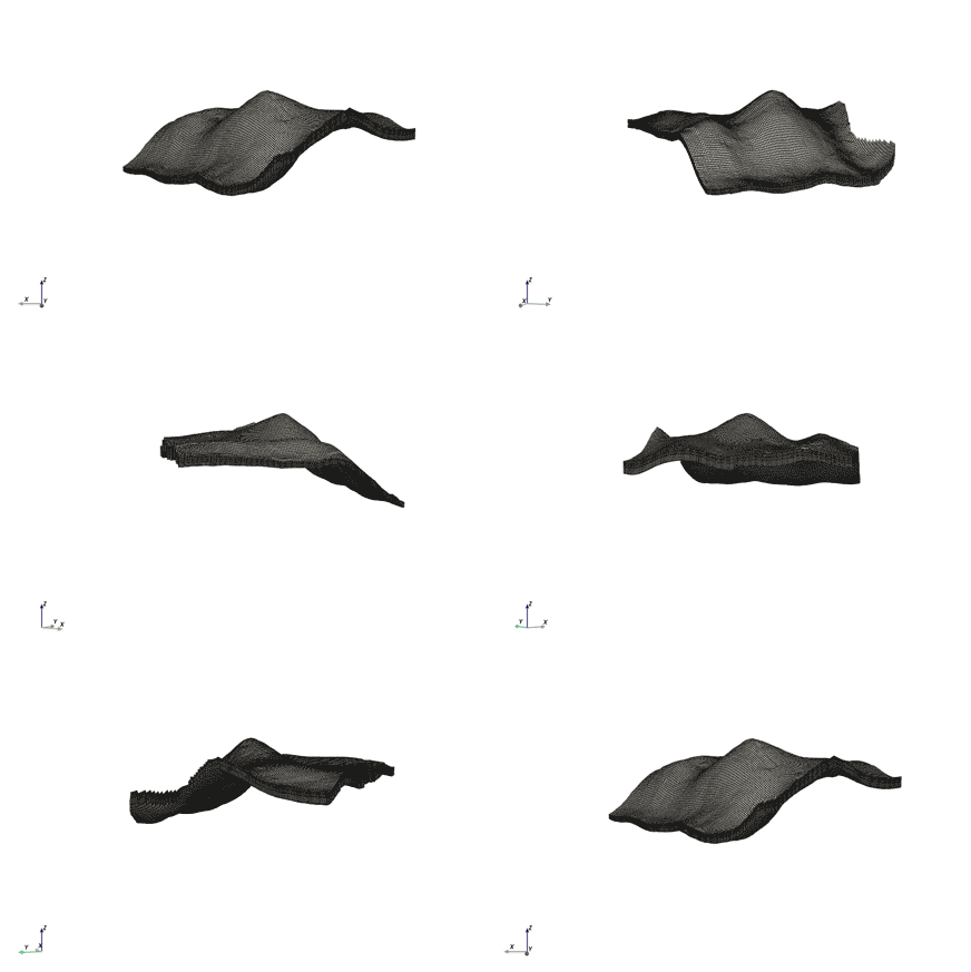
As part of my research on geological CO2 storage, I investigated how different ion activity models influence geochemical predictions in reactive-transport simulations. Although activity models play a fundamental role in calculating aqueous speciation and mineral reactions, their impact on large-scale storage assessments is not always well understood. To explore this, I used a modified version of TOUGHREACT that I had previously extended in Fortran to include the ideal activity model, with the Bunter Sandstone Formation serving as the case study. Before running the simulations, I converted the original Petrel geological model into a workflow that could be used by TOUGHREACT. This involved converting the Petrel grid into VTK format using PyGRDECL and then generating a TOUGHREACT mesh using toughio. I developed six simulation scenarios by combining three initial geochemical equilibrium states (non-equilibrium, semi-equilibrium, and equilibrium) with three activity model formulations (ideal, extended Debye-Huckel, and Pitzer). The objective was to investigate the effects of activity model selection under different geochemical equilibrium assumptions. The results indicated that failing to establish geochemical equilibrium before CO2 injection can lead to a significant underestimation of mineral reactions. In contrast, simulations using the ideal activity model tended to overestimate reaction intensity even when equilibrium conditions were established. Despite this, the ideal model provided sufficient predictive accuracy for large-scale CO2 storage assessments while requiring considerably less computational effort than more complex formulations. To communicate the geological model more effectively, I also created a rotating 3D visualization of the Petrel grid in Python. The animation was later used in a presentation at the 87th EAGE conference and helped illustrate the scale and geometry of the storage formation in a way that static figures could not.

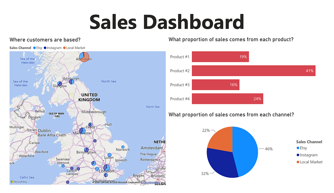
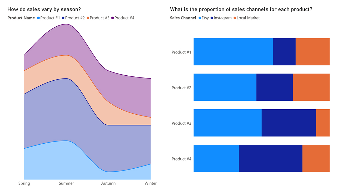
I completed this freelance project for a small business owner in Aberdeen who sold products through local markets as well as online platforms including Instagram and Etsy. The objective was to better understand sales performance and identify potential opportunities for growth using the available transaction data. I used SQL to clean, organize, and analyze the sales records before building an interactive Power BI dashboard to explore trends across products, sales channels, and seasonal patterns. The analysis showed that Product #2 was the strongest contributor to overall revenue and consistently outperformed the other product categories. Sales activity also displayed a clear seasonal pattern, with demand peaking during the summer months. When comparing sales channels, Etsy and Instagram accounted for approximately 78% of total sales, significantly outperforming in-person marketplace sales. This suggested that online channels were the primary drivers of business growth and customer engagement. Based on these findings, I recommended focusing future marketing and sales efforts on online channels and considering the launch of an additional product within the same category as Product #2, particularly during the summer period when demand was highest. At the same time, I avoided drawing conclusions about customer demographics because the available dataset did not contain sufficient customer information to support that type of analysis. This project was a good reminder that useful business insights do not always require large or complex datasets. Even relatively simple sales records can reveal meaningful patterns when the data is cleaned, structured, and analyzed systematically.

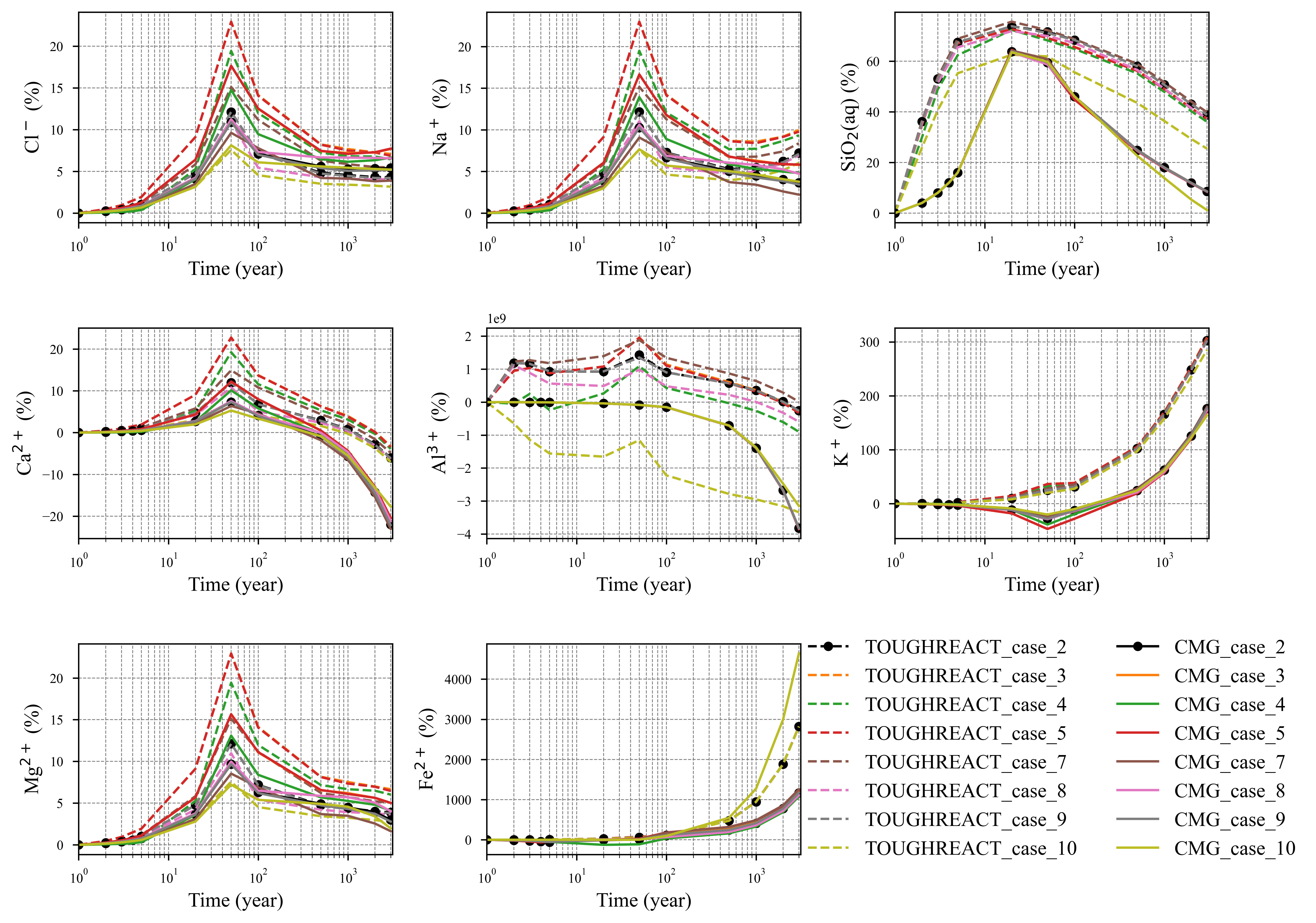
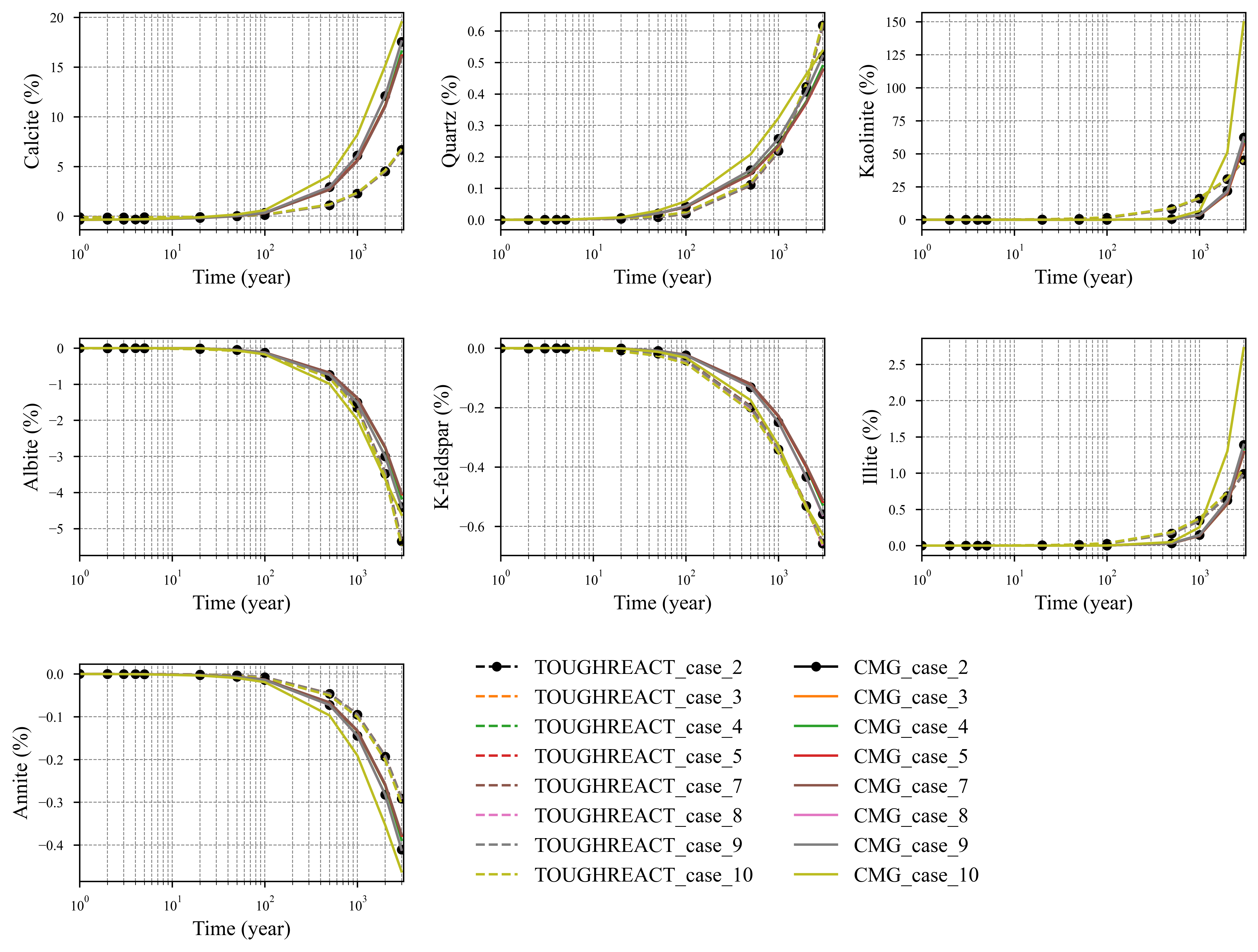
Reactive-transport models contain numerous physical and numerical parameters, many of which can strongly influence simulation outcomes. Understanding which parameters matter most is essential for interpreting results and assessing uncertainty in geological CO2 storage studies. Using the Bunter Sandstone Formation as a case study, I performed a sensitivity analysis with both CMG and TOUGHREACT. The study focused on four key parameters: injection rate, lateral boundary conditions, grid resolution, and reservoir permeability. My goal was to determine how variations in these parameters affected on reactive-transport simulations of CO2 storage, with emphasis on geochemical evolution. To support the analysis, I used the Python post-processing workflows I had developed earlier to automate data extraction and organization. The processed datasets were then analyzed and visualized using Matplotlib. Running the same sensitivity scenarios in two different simulators also allowed me to evaluate how modelling assumptions influenced the results. Both simulators showed similar overall trends despite differences in their underlying implementations. Increasing injection rates gradually over time improved storage capacity while keeping reservoir pressures below fracture limits. Lateral boundary conditions and reservoir permeability were found to be the primary controls on long-term pressure build-up, whereas grid resolution and relative permeability had a stronger influence on CO2 plume migration. One of the most interesting findings was the strong sensitivity of geochemical predictions to grid resolution. Changes in numerical discretization affected the numerical representation of CO2 concentration gradients, which in turn influenced acidity conditions and mineral reactions. The results highlighted how numerical choices can sometimes be just as important as physical parameters when interpreting simulation outcomes. Overall, the study demonstrated the importance of evaluating uncertainty from both geological and numerical sources when assessing the long-term performance of CO2 storage projects.

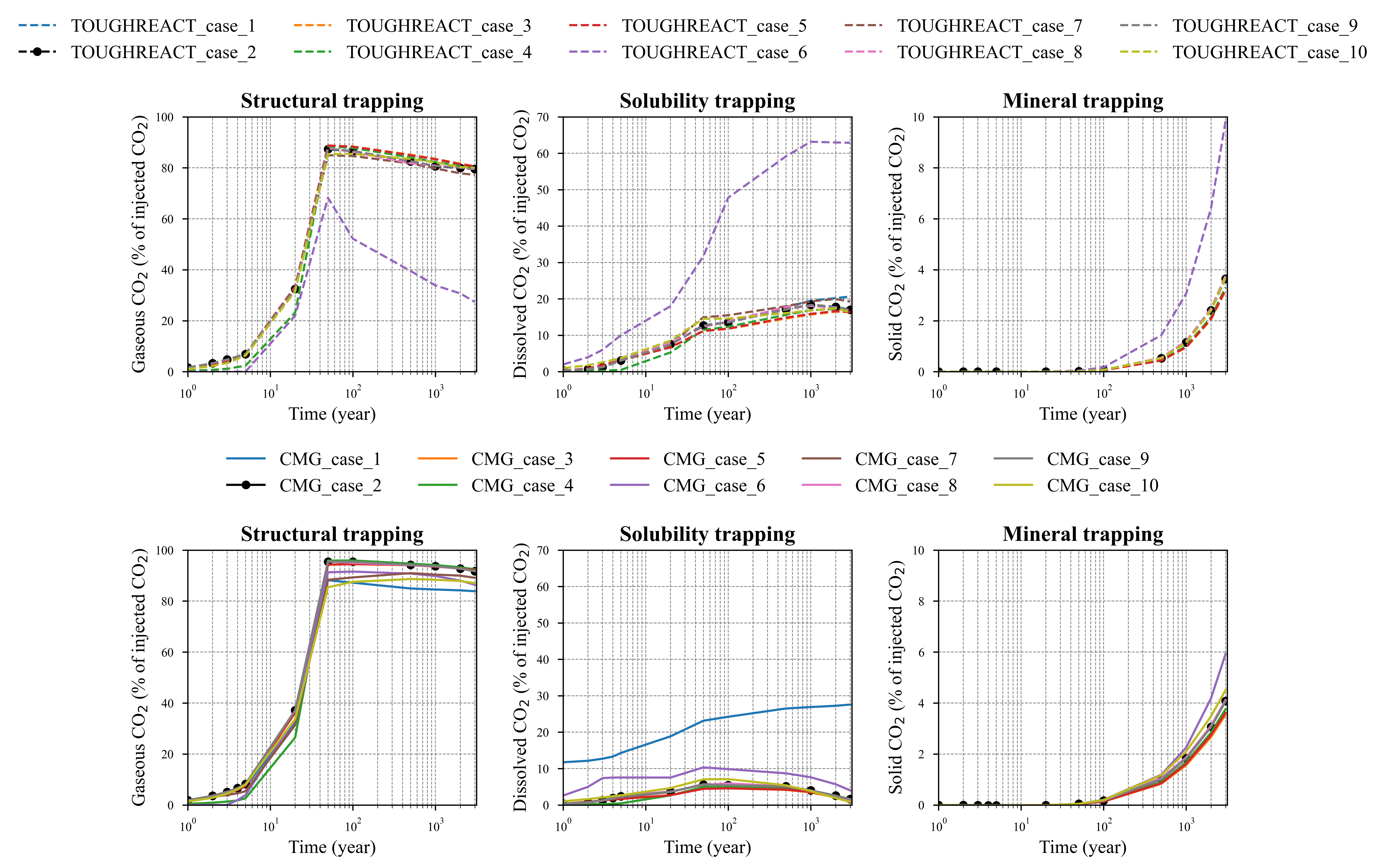
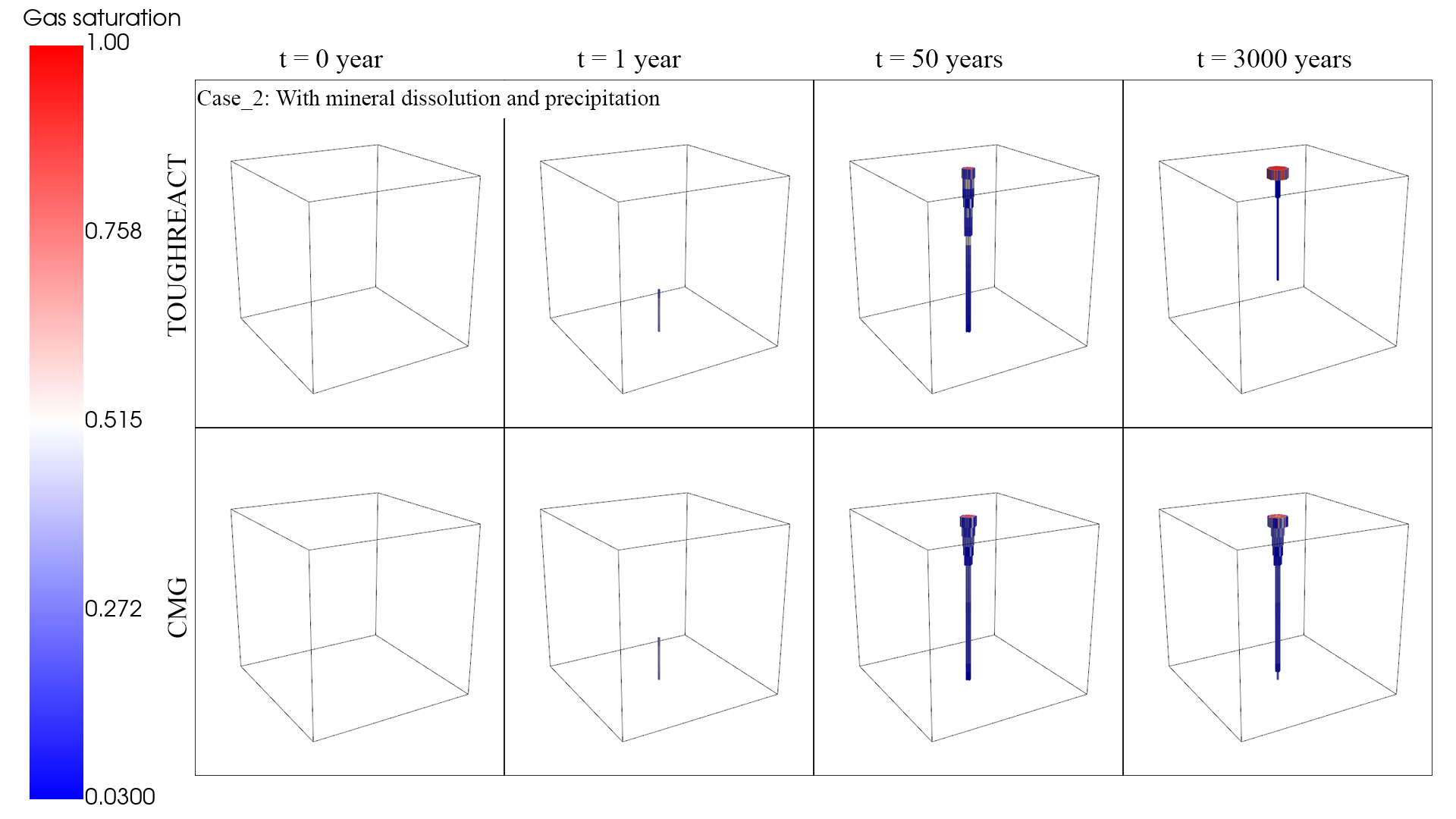
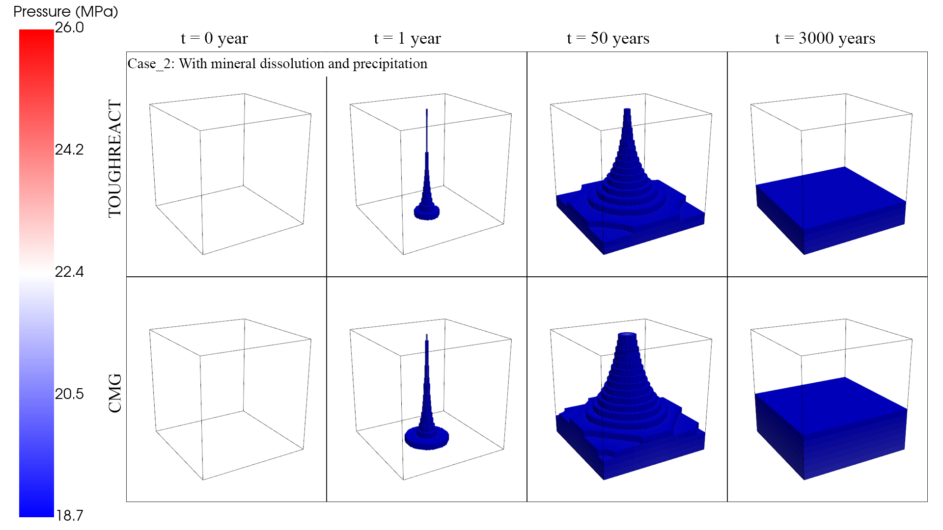
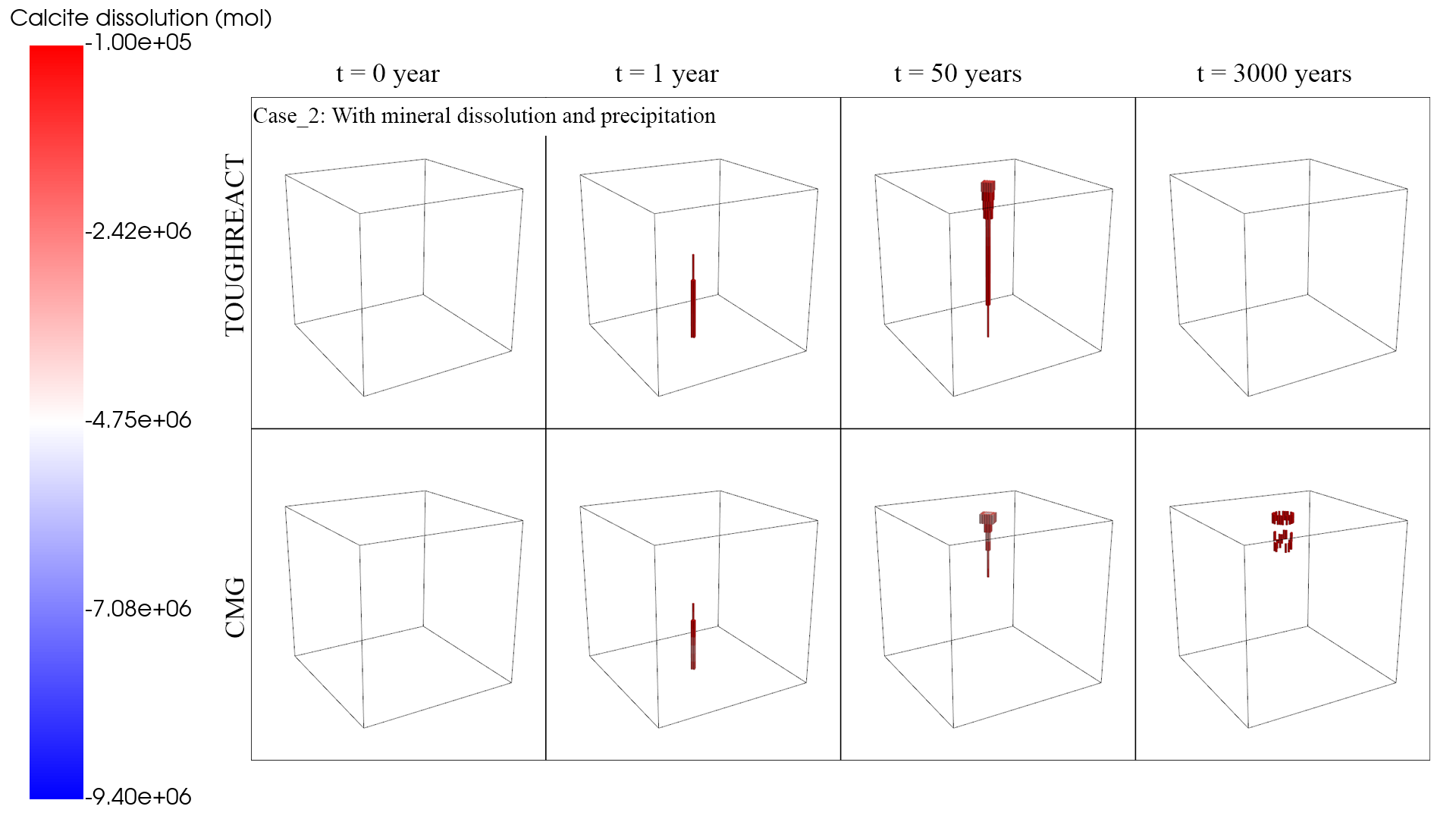
The Bunter Sandstone Formation is widely considered one of the most promising geological CO2 storage candidates in the UK. Despite its potential, uncertainties remain regarding how geochemical reactions evolve during CO2 injection and how consistently different reactive-transport simulators predict these processes. To investigate these questions, I carried out a series of reactive-transport simulations using both CMG-GEM and TOUGHREACT. My objective was to compare storage predictions under harmonised modelling assumptions and identify where the two simulators agreed and where they diverged. The simulation outputs were processed using the Python automation pipelines I had previously developed and visualised in three dimensions using PyVista. Although the models were configured as consistently as possible, they produced systematic differences that could be traced back to their treatment of relative permeability hysteresis and CO2 dissolution. TOUGHREACT generally predicted a larger CO2 plume beneath the caprock, while CMG-GEM predicted greater pressure build-up around the injection well. The geochemical results were more encouraging. Both simulators indicated that calcite dissolution and associated acidity changes remained largely confined to the near-well region, suggesting limited formation-scale geochemical disturbance. Structural trapping dominated the storage mechanism throughout the simulation period, exceeding 80% of the stored CO2 immediately after well shut-in, while mineral trapping contributed approximately 4% of the total storage. This work reinforced the idea that individual simulator predictions should not be interpreted as absolute outcomes. Instead, the range of results produced by multiple simulators can be viewed as a practical uncertainty envelope, providing a more robust basis for assessing long-term CO2 storage performance.

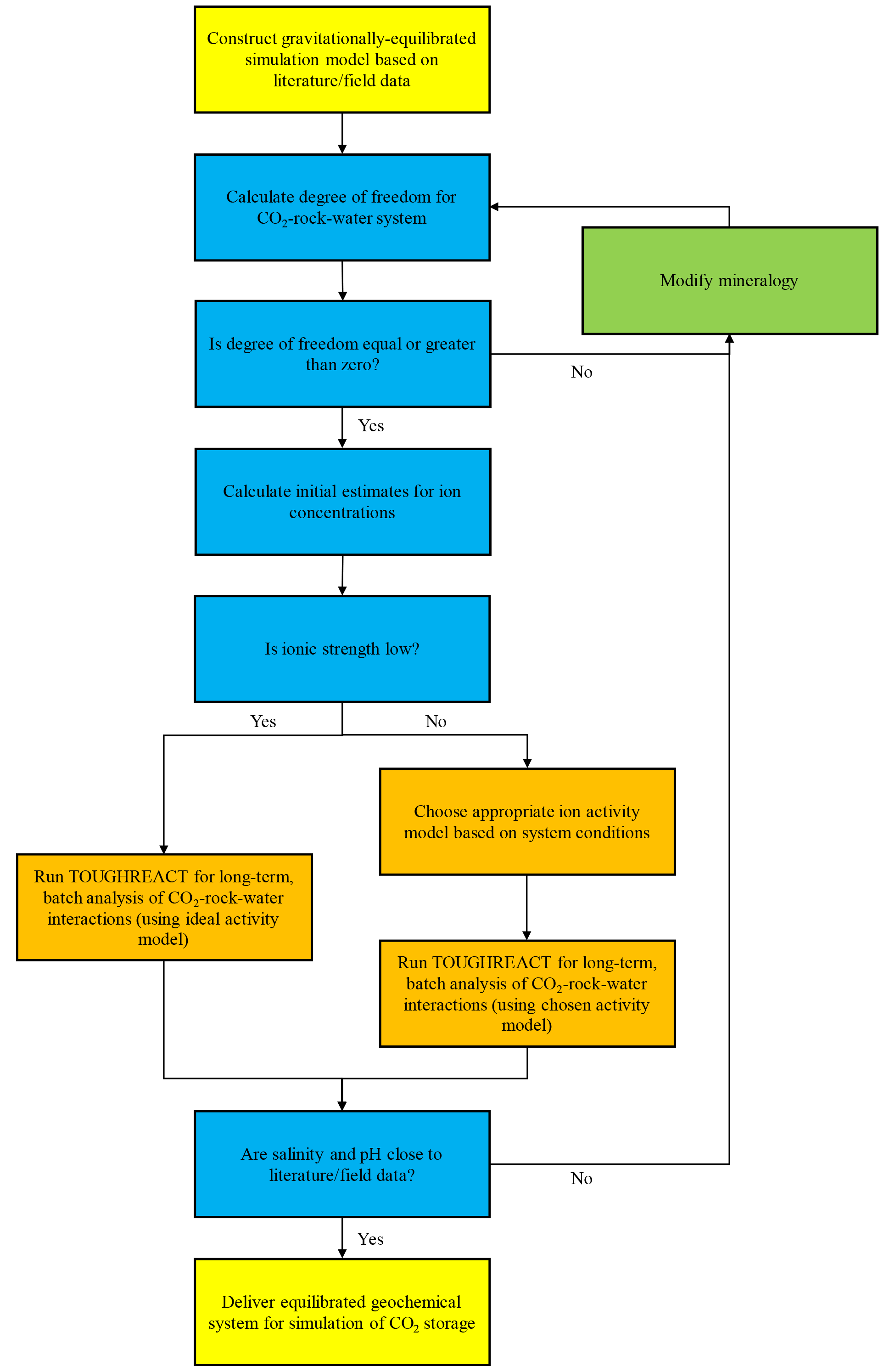
Accurate geochemical initialization is a critical but often overlooked step in reactive-transport modelling. Before simulating CO2 injection, the rock, formation water, and dissolved species should be in chemical equilibrium. If this initial state is not properly established, the simulator may spend much of the calculation correcting artificial imbalances rather than modelling the actual effects of CO2 storage. To address this challenge, I developed a workflow for chemically initializing geological formations prior to CO2 injection. The workflow combines geochemical modelling with thermodynamic equilibrium calculations to generate realistic CO2-rock-water systems that can be used as starting conditions for reactive-transport simulations. The workflow employs ion activity models to calculate equilibrium concentrations while carefully adjusting mineral assemblages to produce salinity and pH values that remain broadly consistent with available laboratory measurements. During this work, I observed that equilibrium concentrations predicted by activity models can differ substantially from short-term experimental observations. These differences are not necessarily errors; rather, they reflect the fact that laboratory experiments are often constrained by practical timescales and may not fully reach long-term equilibrium conditions. The workflow provides a practical bridge between laboratory observations and thermodynamic modelling, helping create more realistic initial conditions for geological CO2 storage simulations. The methodology was later published in a peer-reviewed journal and became a key component of my broader research on reactive-transport modelling.

                        
  # .........................................................
  #  Automation pipeline for processing data from CMG
  # .........................................................

  import numpy as np
  from datetime import datetime


  def import_cmg_data(cell_number, cmg_txt_path):
      nx, ny, nz = cell_number        
      blocks = {}
      current_block = {}
      current_time = None
      first_variable_name = None
      
      i = 0
      j = 0
      k = 0

      skip_until_k = True
      
      if not cmg_txt_path:
          print("dataset not provided")
          return None
          
      else:
          with open(cmg_txt_path, 'r') as f:
              for line in f:
                  line = line.strip()
                  if not line:
                      continue
                  if 'TIME =' in line:
                      skip_until_k = True
                      parts = line.split()
                      if current_time is None:
                          first_timestep = parts[4]
                      difference = datetime.strptime(parts[4], '%Y-%b-%d').year - datetime.strptime(first_timestep, '%Y-%b-%d').year
                      current_time = round(float(difference))
                      if current_time not in blocks:
                          blocks[current_time] = {}
                      continue
                  elif 'RESULTS PROP' in line and 'Units:' in line:
                      start = line.find('RESULTS PROP') + len('RESULTS PROP')
                      end = line.find('Units', start)
                      variable_name = line[start:end].strip()
                      if first_variable_name is None:
                          first_variable_name = variable_name
                      continue
                  elif 'K =' in line:
                      skip_until_k = False
                      parts = line.replace("**", "").replace(" ", "").split(",")
                      k = int(parts[0].split("=")[1])
                      j = int(parts[1].split("=")[1])
                      i = 1
                      continue
                  elif not skip_until_k:
                      parts = line.split()
                      if 'index' not in blocks[current_time]:
                          blocks[current_time]['index'] = []
                      if variable_name not in blocks[current_time]:
                          blocks[current_time][variable_name] = []
                      for value in parts:
                          if variable_name == first_variable_name:
                              blocks[current_time]['index'].append((i, j, k))
                          blocks[current_time][variable_name].append(float(value))
                          i += 1
              
          for timestep, block in blocks.items():
              for name, values in block.items():
                  block[name] = np.array(values)

      print('Time steps in cmg file:', list(blocks.keys()))
      print('Variables in cmg file:', list(next(iter(blocks.values())).keys()))
      print('===================================================================')
      return blocks
                        
                      

                        
  # .........................................................
  #  Automation pipeline for processing data from TOUGHREACT
  # .........................................................

  import numpy as np


  def import_toughreact_data(cell_number, *address):
      flow_tec_path = address[0]
      
      if len(address) > 1:
          mineral_tec_path = address[1] 
      else:
          mineral_tec_path = None
      
      if len(address) > 2:
          concentration_tec_path = address[2] 
      else:
          concentration_tec_path = None

      nx, ny, nz = cell_number
      
      def _read_tec(filepath):
          
          blocks = {}
          current_block = {}
          current_time = None
          var_names = []
          with open(filepath, 'r') as f:
              for line in f:
                  line = line.strip()
                  if not line:
                      continue
                  if 'Variables=' in line:
                      # extract variable names in quotes
                      parts = line.replace('Variables=', '').split('"')
                      for i in parts:
                          if i and not i.isspace():
                              var_names.append(i)
                  elif 'Zone T=' in line:
                      # save previous block
                      if current_time is not None and current_block:
                          blocks[current_time] = current_block
                      # reset
                      current_block = {}
                      for name in var_names:
                          current_block[name] = []    
                      # parse time between T=" and " sec
                      start = line.find('Zone T=') + len('Zone T=')
                      end = line.find('sec', start)
                      t = line[start:end].strip().strip('"')
                      # handle zero-time special-case
                      if t == '1.00000000E+00':
                          t = '0.00000000E+00'
                      current_time = round(float(t)/3.15360000E+07)
                  else:
                      # data lines
                      parts = line.split()
                      if current_time is not None and len(parts) == len(var_names):
                          for i, name in enumerate(var_names):
                              current_block[name].append(float(parts[i]))
          # final block
          if current_time is not None and current_block:
              blocks[current_time] = current_block
          # reshape and flatten
          for timestep, block in blocks.items():
              for name, values in block.items():
                  arr = np.array(values).reshape((nx, ny, nz), order='C')
                  block[name] = arr.flatten(order='F')
          return blocks

      flow_blocks = _read_tec(flow_tec_path)
      blocks = flow_blocks
      
      if mineral_tec_path:
          mineral_blocks = _read_tec(mineral_tec_path)
          for timestep in mineral_blocks:
              if timestep in blocks:
                  blocks[timestep].update(mineral_blocks[timestep])
              else:
                  blocks[timestep] = mineral_blocks[timestep]
      else:
          mineral_blocks = None
          print("Mineral file not provided")

      if concentration_tec_path:
          concentration_blocks = _read_tec(concentration_tec_path)
          for timestep in concentration_blocks:
              if timestep in blocks:
                  blocks[timestep].update(concentration_blocks[timestep])
              else:
                  blocks[timestep] = concentration_blocks[timestep]
      else:
          concentration_blocks = None
          print("Concentration file not provided")

      
      
      print('Time steps in tough file:', list(blocks.keys()))
      print('Variables in tough file:', list(next(iter(blocks.values())).keys()))
      print('===================================================================')
    
      return blocks
                        
                      

Reactive-transport simulations generate a huge amount of output data. A single simulation can contain thousands of grid cells, dozens of variables, and hundreds of time steps, making manual processing both inefficient and error-prone. Since I was comparing results from CMG-GEM and TOUGHREACT, I also needed a consistent workflow that could handle outputs from both simulators in the same way. To solve this problem, I developed a set of Python automation pipelines for importing, organizing, and processing simulation results. The workflow begins by reading raw simulator output files line by line and converting unstructured text into a format suitable for analysis. This includes identifying simulation time steps, extracting reservoir properties, mapping values to their corresponding grid cells, and preserving spatial indexing information. The main functions, import_cmg_data() and import_toughreact_data(), automatically parse simulator outputs and store the results in structured numerical arrays. The workflow also identifies available variables, tracks temporal changes, and creates a consistent data structure regardless of the source simulator. Building these tools significantly reduced the amount of time required for post-processing and eliminated many repetitive manual tasks. More importantly, it improved the reproducibility of my work by ensuring that every simulation was processed using the same methodology. The processed datasets later became the foundation for both 2D and 3D visualization workflows, allowing me to analyze CO2 migration, geochemical evolution, pressure behavior, and mineral reactions across multiple simulation scenarios.

                        
  c .........................................................
  c  Incorporating specific relative permeability fucntions
  c .........................................................
  c .........................................................
  c                      MODULE_t2f
  c .........................................................
  c
        SUBROUTINE INPUT
  c
  c
  c-----READ ALL DATA PROVIDED THROUGH THE INPUT FILE.
  c
  c
  c-----THIS ROUTINE COMPUTES RELATIVE PERMEABILITIES FOR LIQUID
  c     AND GASEOUS PHASES.
  c
  c
        implicit real*8  (a-h,o-z)
        implicit integer*8 (i-n)
        INCLUDE 'flowpar_v4.inc'
  c
        COMMON/P3/DELX((MNK+1)*MNEL)
        COMMON/RPCAP/IRP(MAXMAT),RP(7,MAXMAT),ICP(MAXMAT),CP(7,MAXMAT),
      XIRPD,RPD(7),ICPD,CPD(7)
  !els12/02/15 add new pcap parameters
        common/rpcap2/cpsavpar(6,maxmat),rpsavpar(12,maxmat)
  c       Added definitions below
        double precision sg,repl,repg,sg0
        integer*8 nmat,k,nloc
  c
        SAVE ICALL
        DATA ICALL/0/
        ICALL=ICALL+1
        IF(ICALL.EQ.1) WRITE(11,899)
  c 899 FORMAT(6X,'RELP     1.0      25 JANUARY   1990',6X,
  c 899 FORMAT(6X,'RELP     1.0      23 November  1994',6X,
  c  899 FORMAT(6X,'RELP     1.0      26 July      1995',6X,
  !els11/30/15  899 FORMAT(6X,'RELP     1.1      20 March     2009',6X,
    899 FORMAT(6X,'RELP     1.11      30 November   2015',6X,
      X'LIQUID AND GAS PHASE RELATIVE PERMEABILITIES AS FUNCTIONS',
      X' OF SATURATION'/
      x47X,'for IRP=7, use Corey-krg when RP(4).ne.0, with Sgr',
      x' = RP(4)')
  c
        SL=1.d0-SG
  c      GOTO(10,11,12,12,13,14,15,16),IRP(NMAT)
  c Added new option 11, from ITOUGH (S. Finsterle)
        GOTO(10,11,12,12,13,14,15,16,17,18,19),IRP(NMAT)
    10 CONTINUE
  c-----LINEAR FUNCTIONS.
  c
  c     CHECK IF INCREMENT NEEDS TO BE ADJUSTED AT LOWER LIQUID CUTOFF.
        IF(K.NE.3) GOTO 20
        IF((SL-RP(1,NMAT))*(1.d0-SG0-RP(1,NMAT)).GE.0.d0) GOTO 20
  c     ADJUST INCREMENT.
        DELX(NLOC+2)=-DELX(NLOC+2)
        SG=SG0+DELX(NLOC+2)
        SL=1.d0-SG
    20 CONTINUE
  c
  !els12/02/15      REPL=(SL-RP(1,NMAT))/(RP(3,NMAT)-RP(1,NMAT))
        REPL=(SL-RP(1,NMAT))/rpsavpar(1,nmat)
        IF(SL.GE.RP(3,NMAT)) REPL=1.d0
        IF(SL.LE.RP(1,NMAT)) REPL=0.d0
  !els12/02/15      REPG=(SG-RP(2,NMAT))/(RP(4,NMAT)-RP(2,NMAT))
        REPG=(SG-RP(2,NMAT))/rpsavpar(2,nmat)
        IF(SG.GE.RP(4,NMAT)) REPG=1.d0
        IF(SG.LE.RP(2,NMAT)) REPG=0.d0
  c
        RETURN
  c
    11 CONTINUE
  c-----RELATIVE PERMEABILITY OF PICKENS ET AL.
  c
        REPG=1.d0
        REPL=(1.d0-SG)**RP(1,NMAT)
  c
        RETURN
  c
    12 CONTINUE
  c-----COREY@S OR GRANT@S CURVES.
  c
  !els12/02/15      SSTAR=(SL-RP(1,NMAT))/(1.d0-RP(1,NMAT)-RP(2,NMAT))
        SSTAR=(SL-RP(1,NMAT))/rpsavpar(1,nmat)
        REPL=SSTAR**1.70E0
        REPG=0.50E0*(1.d0-SSTAR**1.2)*(1.d0-SSTAR)**0.40E0
        IF(SG.GE.RP(2,NMAT)) GOTO 50
        REPG=0.d0
        REPL=1.d0
        GOTO 102
  !els12/02/15   50 IF(SG.LT.(1.d0-RP(1,NMAT))) GOTO 102
    50 IF(SG.LT.rpsavpar(2,nmat)) GOTO 102
        REPL=0.d0
        REPG=1.d0
    102 CONTINUE
        IF(IRP(NMAT).EQ.4) REPG=1.d0-REPL
        RETURN
  c
    13 CONTINUE
  c-----BOTH PHASES ARE PERFECTLY MOBILE.
  c
        REPL=1.d0
        REPG=1.d0
  c
        RETURN
    14 CONTINUE
  c-----RELATIVE PERMEABILITIES OF FATT AND KLIKOFF (1959), AS REPORTED
  c     BY K. UDELL (BERKELEY, 1982).
  c
        SS=0.d0
  !els12/02/15      IF(SL.GT.RP(1,NMAT)) SS=(SL-RP(1,NMAT))/(1.d0-RP(1,NMAT))
        IF(SL.GT.RP(1,NMAT)) SS=(SL-RP(1,NMAT))/rpsavpar(1,nmat)
        REPL=SS**3
        REPG=(1.d0-SS)**3
        RETURN
  c
    15 CONTINUE
  c-----RELATIVE PERMEABILITY OF VAN GENUCHTEN, SOIL SCI. SOC. AM. J. 44,
  c     PP. 892-898, 1980.
  c
        IF(SL.GE.RP(3,NMAT)) GOTO 150
  !els12/02/15      SS=(SL-RP(2,NMAT))/(RP(3,NMAT)-RP(2,NMAT))
        SS=(SL-RP(2,NMAT))/rpsavpar(1,nmat)
        REPL=0.d0
  c
                        
                      

                        
  c .........................................................
  c  Incorporating ideal activity model
  c .........................................................
  c .........................................................
  c                      MODULE_geochem
  c .........................................................
  c
        subroutine hkfpar(T,tk,adh,bdh,bi,bil)
  c
  c
  c
  c   bhat NaCl (b NaCl = bhat/(2.303RT)) from Table 29 (bi here)
  c   b Na+Cl- from Table 30 (bil here)
  c   A and B Debye-Huckel (adh and bdh) from Table 1 (cols. 3 and 4)
  c
  c  Polynomial regression coefficients a, b, c, d, e, and f are
  c  stored in data statements below to calculate parameters as:
  c     parameter(T) = a + b*T + c*T + d*T**2 + e*T**3 + f*T**4
  c  where T is temperature in C.
  c
  c  These are good for the range 0 to 300 C, BUT(!) the data
  c  available to fit bi and bil did not go down to T = 0 C
  c  (first point at 25 C) so the extrapolation may not be too good
  c  below 25 C for bi and bil (A and B data cover the entire range),
  c  but I checked that the extrapolated bi and bil values below
  c  25 C vary smoothly down to 0 C.
  c
  c  Note the following units:
  c    aft    yields adh in kg**0.5 mol**(-0.5)
  c    bft    yields bdh in kg**0.5 mol**(-0.5) Anstrom**(-1)
  c    bift   yields bihat(NaCl) in kg/mol * 1e+3
  c    bilft  yields bil (Na+Cl-) in kg/mol * 1e+2
  c
        implicit double precision (a-h,o-z)
        implicit integer*8 (i-n)
        double precision aft(5), bft(5), bift(5), bilft(5)
        double precision t,tk,adh,bdh,bi,bil,bihat
  c
        data aft/0.49276542d+00,0.31857945d-03,0.11628933d-04,
      &   -0.52038832d-07,0.12633045d-09/
        data bft/0.32476341d+00,0.12018502d-03,0.79530646d-06,
      &   -0.30410531d-08,0.56931304d-11/
        data bift/0.26538636d+01,-0.52889569d-02,-0.11009615d-03,
      &    0.46820513d-06,-0.11104895d-08/
        data bilft/-0.14769091d+02,0.22563951d+00,-0.10225385d-02,
      & 0.30349650d-05,-0.35468531d-08/
  c
        func(a,b,c,d,e,T) = a+(b+(c+(d+e*T)*T)*T)*T
  c
        SAVE ICALL
        DATA ICALL/0/
        ICALL=ICALL+1
        IF(ICALL.eq.1) WRITE(11,"(
      & 6x,'hkfpar     2.1    12 September  2013',
      & 6x,'Assigns data for calculation of Debye-Huckel parameters'
      & )")
  c
        adh=func(aft(1),aft(2),aft(3),aft(4),aft(5),T)
        bdh=func(bft(1),bft(2),bft(3),bft(4),bft(5),T)
        bihat=func(bift(1),bift(2),bift(3),bift(4),bift(5),T)*1.d-3
        bi=bihat/(4.57061d0*tk)  ![kg cal/mol]
        bil=func(bilft(1),bilft(2),bilft(3),bilft(4),bilft(5),T)*1.d-2
  c
        return
        end
  c
  c-------------------------------------------------------------------------------
  c
          subroutine dh_hkf81(no_ch,tk2,adh,bdh,bi,bil,str,gamp,gams,
      &       cs,ct,u2,cpw,xh2o,gampdl,gamsdl,
      &       mstar,stroot)

  c
  C****************** Calculate activity coefficient of aqueous species ************
  C   idryout is for dryout without update activity coefficients 0 and 1 normal, 2, skip
  CC
  c  This routine computes activity coefficients of aqueous species
  c  and the activity of water using pitzer model or an extended DH model according

  c  to a user-specified ionic strength threshold and a user option.  The extended

  c  DH model uses equations and parameters given in Helgeson, Kirkham and

  c  Flowers, 1981, A.J.S. p.1249-1516. Also computes neutral species activities
  c  from Setchenov equation (Langmuir 1997, Aqueous Environmental
  c  Geochemistry, Prentice Hall, p. 144).
  c  Charged species: individual ion activity coefficients calculated from:
  c     equation 298 (which includes 121, 122, 129, 130, 169, 170 and 297)
  c      - uses true ionic strenght.
  c     use bhat NaCl (b NaCl = bhat/(2.303RT)) from Table 29 (bi here)
  c     use b Na+Cl- from Table 30 (bil here)
  c     use Rej from Table 3 (input in thermodynamic database as
  c       a0 variable, but note that values are NOT a0 values)
  c     use A and B Debye-Huckel (adh and bdh) from Table 1 (cols. 3 and 4)
  c     caclulate a0 from input Rej values and eq. 125,
  c       assuming other dominant anion (for cations) is Cl- (rej=1.81 A)
  c       and cation (for anions) is Na+ (rej=1.91 A)
  c
  c  Activity of water calculated from:
  c     osmotic coefficient using equation 190 and same parameters
  c       as above, assuming similar simplifications as done for
  c       the calculation of activity coefficients, but using
  c       stoichiometric ionic strength.
  c     equation 106 relating activity of water to the osm. coef.
  c
  c  Regression coefficients a, b, c, d, e to obtain A, B, bi abd bil
  c  parameter as a function of temperature were calculated using
  c  4th order polynomials as follow:
  c        f(T) = a + b*T + c*T**2 + d*T**3 + e*T**4
  c
  c  Neutral species: assume gamma = 1 or,
  c  for weak acids and dissolved gases:
  c    log(activity coef)=sltout*ionic strength
  c    where sltout is input in a0 variable as 100+sltout
  c    For now, no temperature dependence on sltout is assumed as
  c    the effect is small compared to variation of solubility (K) with temp.
  c
        implicit double precision (a-h,o-z)
        implicit integer*8 (i-n)
        include 'flowpar_v4.inc'
        include 'chempar_v4.inc'
        include 'common_v4.inc'
        integer*8 no_ch
        integer*8 nprsec,ncp,niis,iis
        double precision lambda, lambd2, mstar, mchr
        double precision bdhstrt,bdhstr2,bdh3str2,adhstrt
        double precision cpgmdms,bistr,bistr2,gamlog
        double precision cpion(maqt)
        double precision adh,bdh,bi,bil,str,tk2
        double precision stroot,stroo2,sum,sum2,str2,summt,capgam
        double precision cpw(mpri),xh2o
        double precision gamp(mpri),gams(maqx)
  cels5/1/14 keep versions that don't have to be logged
        double precision gampdl(mpri),gamsdl(maqx)
        double precision cs(maqx),u2(mpri),ct(mtot)
  !els4/5/16      double precision gamln,gsalt,sltout,cpwmax
        double precision gamln,gsalt,sltout
        parameter(CC=-1.0312d0,FF=0.0012806d0,GG=255.9d0,EE=0.4445d0,
      +   HH=-0.001606d0)
  c
  c
  c-22-March-2000------ salting out effect, Wolery's EQ3NR Eq. (91)
  c
        SAVE ICALL
  cpitz      SAVE gam
        DATA ICALL/0/
  ccc      data amwh2o/18.0152d0/

        ICALL=ICALL+1
        IF(ICALL.EQ.1) then
        WRITE(11,899)
  !els4/5/16  899  FORMAT(6X,'dh_hkf81 2.2      1 May 2014',6X,
    899  FORMAT(6X,'dh_hkf81 2.3     5 Apr 2016',6X,
      X'Calculate activity coefficient of aqueous species')
  c
        endif
  C
  cels5/22/12 moved initialization outside of icall loop
  c
  c ns-jan08     Initializes gammas
  cels5/1/14 initial dlog of gamma
        do i=1,npri+1   !ns12/2017 add 1 to store gamma for water
          gamp(i) = 1.d0
          gampdl(i) = 0.d0
        enddo
  c
        do i=1,naqx
          gams(i) = 1.d0
          gamsdl(i) = 0.d0
        enddo
  c
                        
                      

TOUGHREACT is a non-isothermal, multi-component, multi-phase reactive-transport simulator widely used for modelling subsurface processes such as geological CO2 storage, geothermal systems, and environmental remediation. It can simulate both batch geochemical reactions and three-dimensional reactive flow while accounting for mineral dissolution, precipitation, and aqueous speciation. While using TOUGHREACT for my research, I found two limitations that made direct comparison with CMG-GEM difficult. The first was the absence of an ideal activity model within the geochemical framework. The second was the lack of support for tabular or functional relative permeability inputs. These differences affected the ability to align modelling assumptions across the two simulators and isolate the causes of discrepancies in their predictions. To address this, I modified the Fortran source code of TOUGHREACT version 4.13. The implementation involved extending the relative permeability routines in t2f_v4.f and modifying the geochemical calculations in geochem_v4.f. The goal was not simply to add new functionality, but to create a more consistent basis for cross-simulator comparison. The updated version allowed me to run simulations using modelling assumptions that more closely matched those available in CMG-GEM. This made it possible to evaluate differences arising from the numerical and physical formulations of the simulators rather than from incompatible input options. The work also gave me practical experience working with a large scientific codebase and translating theoretical modelling requirements into production-level Fortran code.

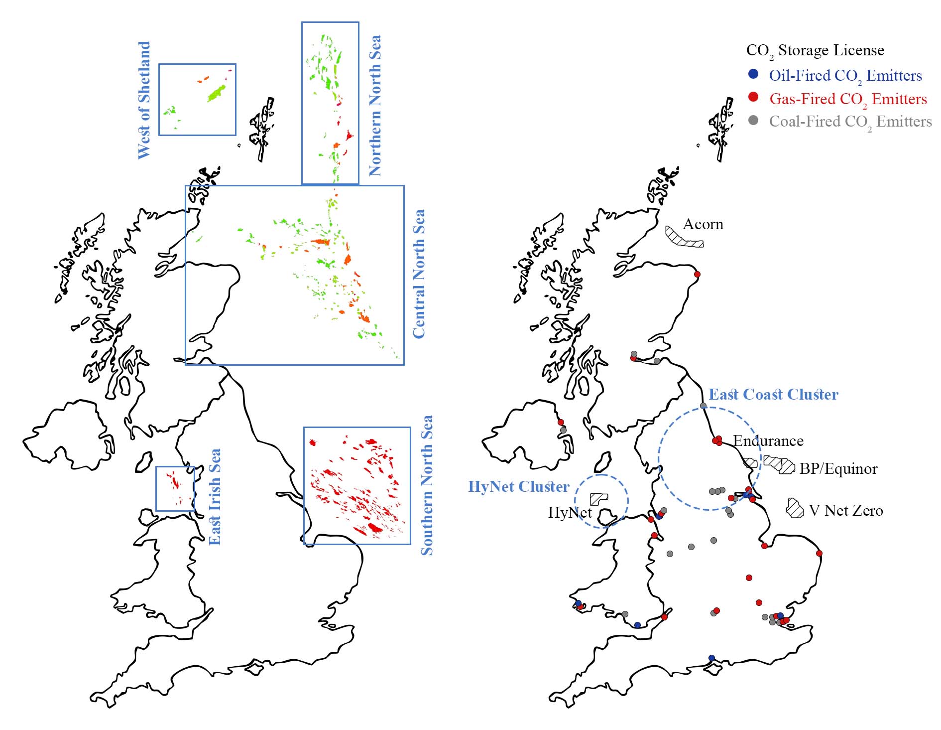
Finding suitable CO2 storage sites starts with identifying geological formations that can safely contain CO2 over very long timescales. Geological storage remains the most practical option because subsurface formations have already demonstrated their ability to trap hydrocarbons for millions of years, and a large amount of geological data is available from decades of oil and gas exploration. As part of a four-stage site-screening workflow, I collected and integrated publicly available GIS datasets to evaluate potential CO2 storage opportunities across the UK. The project involved combining geological, geographical, and infrastructure datasets into a single mapping framework that could be used to compare potential storage locations. The resulting maps highlighted the spatial distribution of prospective storage sites and helped narrow down areas for further investigation. This work formed the basis of a presentation that I delivered at the 3rd ICESF conference.